9_ctx_3region_DEGs_expression_in_cc

[1]:

import pandas as pd
import scanpy as sc
from scipy.spatial import cKDTree
from tqdm import tqdm
import matplotlib.pyplot as plt

import warnings
import seaborn as sns
import matplotlib as mpl
mpl.rcParams['pdf.fonttype'] = 42
mpl.rcParams['ps.fonttype'] = 42

warnings.filterwarnings('ignore')

/mnt/Data16Tc/home/haichao/anaconda3/envs/SpaCon_test/lib/python3.8/site-packages/tqdm/auto.py:21: TqdmWarning: IProgress not found. Please update jupyter and ipywidgets. See https://ipywidgets.readthedocs.io/en/stable/user_install.html
  from .autonotebook import tqdm as notebook_tqdm

gene exp data

[3]:

adata_in = sc.read_h5ad('/mnt/Data16Tc/home/haichao/code/SpaCon/Data/N_20231213_zxw/mouse_3/adata_processed.h5ad')
allen_region = pd.read_csv('/mnt/Data16Tc/home/haichao/code/SpaCon/Data/N_20231213_zxw/mouse_3/allen_region.csv')
adata_in.obs['region'] = allen_region['region'].values
meta = pd.read_csv('/mnt/Data16Tc/home/haichao/code/SpaCon/Data/N_20231213_zxw/mouse_3/cell_metadata_with_cluster_annotation.csv')
meta = meta.set_index('cell_label')
meta = meta.loc[adata_in.obs.index.to_list()]
adata_in.obs['cell_type'] = meta['class'].to_list()

adata_out = sc.read_h5ad('/mnt/Data18Td/Data/haichao/merfish_raw_data_zxw3/out_cell_adata/adata_out_cell_distance_q0.3/after_qc/Zhuang-ABCA-3.001.h5ad')
adata_out.obs['region'] = adata_in.obs.loc[adata_out.obs_names]['region'].values

adata_in = adata_in[adata_in.obs['cell_type'].str.contains('Glut')]
adata_out.obs

[3]:

	totalRNA	brain_section_label	x	y	z	n_genes_by_counts	total_counts	region
100008170567769574864159172860058606533	175	Zhuang-ABCA-3.001	19.063883	33.423346	54.106801	100	175	MOB
100019036144713180485707288452329906643	373	Zhuang-ABCA-3.001	44.290637	63.872748	53.902462	189	373	NDB
10002377904544842423531242460024745973	277	Zhuang-ABCA-3.001	63.860525	7.998013	54.043841	126	277	RSPd2/3
100027648052649525810014127621472143070	435	Zhuang-ABCA-3.001	113.480480	41.056674	54.349928	165	435	arb
100029875144524072265954931895494067096	60	Zhuang-ABCA-3.001	11.572676	37.921554	54.370336	39	60	MOB
...	...	...	...	...	...	...	...	...
99961718914838042706216314325649765172	627	Zhuang-ABCA-3.001	113.199100	23.661374	54.096322	157	627	CENT3
9996242280180655885872867452807576494	157	Zhuang-ABCA-3.001	86.896566	18.326938	54.027272	100	157	SCop
999921392501518309214993564089572563	97	Zhuang-ABCA-3.001	21.082878	31.635078	54.090905	67	97	ORBm1
99995909784199304193294645747252265238	154	Zhuang-ABCA-3.001	111.605478	22.417974	54.070819	93	154	CENT3
99996568769251334694329666788053033728	200	Zhuang-ABCA-3.001	112.945756	31.433985	54.093405	95	200	CENT3

83602 rows × 8 columns

[4]:

gene_com = list(set(adata_in.var_names) & set(adata_out.var_names))
adata_in = adata_in[:, gene_com]
adata_out = adata_out[:, gene_com]

[5]:

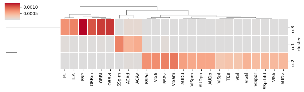
ctx2cc_conn_cluster_mean = pd.read_csv('./ctx_cc_conn_filtered.csv', index_col=0)
sns.clustermap(ctx2cc_conn_cluster_mean, cmap='coolwarm', center=0, figsize=(10, 3), linewidths=0.05, linecolor='white')

[5]:

<seaborn.matrix.ClusterGrid at 0x7f887404b310>

_images/9_ctx_3region_DEGs_expression_in_cc_5_1.png

[6]:

adata_ctx = adata_in[adata_in.obs['region'].str.startswith(tuple(ctx2cc_conn_cluster_mean.columns))]
adata_ctx

[6]:

View of AnnData object with n_obs × n_vars = 67823 × 1111
    obs: 'brain_section_label', 'x', 'y', 'z', 'x_ccf', 'y_ccf', 'z_ccf', 'region', 'cell_type'

[12]:

ctx1 = ['FRP', 'ORBl', 'ORBvl', 'ORBm', 'PL', 'ILA']
ctx2 = ['SSp-m', 'ACAd', 'ACAv']
ctx3=['RSPv','RSPd', 'VISpm', 'VISa', 'VISam', 'SSp-bfd', 'VISpor', 'VISli', 'TEa', 'VISpl', 'VISl', 'AUDv', 'VISal', 'AUDpo', 'AUDp', 'AUDd']
adata_ctx.obs['cc_ctx'] = None
adata_ctx.obs.loc[adata_ctx.obs['region'].str.startswith(tuple(ctx1)), 'cc_ctx'] = 'ctx1'
adata_ctx.obs.loc[adata_ctx.obs['region'].str.startswith(tuple(ctx2)), 'cc_ctx'] = 'ctx2'
adata_ctx.obs.loc[adata_ctx.obs['region'].str.startswith(tuple(ctx3)), 'cc_ctx'] = 'ctx3'
adata_ctx = adata_ctx[adata_ctx.obs['cc_ctx'].notna()]

[ ]:

adata_cc = adata_out[adata_out.obs['region'].str.startswith('cc')]
tmp = adata_cc.copy()
idx = []
cc_cluster_by_conn = pd.read_csv('./cc_cluster_by_conn.csv', index_col=0)
coordinate = cc_cluster_by_conn[['x', 'y']].values
kdtree = cKDTree(coordinate)
for coord in tqdm(adata_cc.obs[['x', 'y']].values):
    _, nearest_index = kdtree.query(coord)
    idx.append(nearest_index)
plt.figure(figsize=(9,5))
### match the cc cluster
adata_cc.obs['NT_index'] = idx
adata_cc.obs['cc'] = cc_cluster_by_conn.loc[adata_cc.obs['NT_index']]['c'].values
adata_cc = adata_cc[adata_cc.obs['cc'].notna()]
adata_cc.obs['cc'] = 'cc'+((adata_cc.obs['cc']).astype(int)+1).astype(str)
#### plot
categories = adata_cc.obs['cc'].unique()
# plt.scatter(adata_out.obs['x'], adata_out.obs['y'], s=1, c='#d3d3d3')
plt.scatter(tmp.obs['x'], tmp.obs['y'], s=20, c='#8f8f8f')
# plt.scatter(tmp.obs['x'], tmp.obs['y'], s=20, c='#d3d3d3')

cm = ['#ff7f0e', '#2ca02c', '#2377b4']
# cm = ['#6597b9', '#6bad6b', '#e9a161']
i=0
for category in categories:
    subset = adata_cc[adata_cc.obs['cc'] == category]
    plt.scatter(subset.obs['x'], subset.obs['y'], label=category, s=20, c=cm[i])
    # print(f'cc_{int(category)}')
    i=i+1
plt.legend()
plt.gca().invert_yaxis()
# plt.savefig('cc_area.png', dpi=600)
# plt.savefig('./cc/cc1_cc2_cc3.pdf', format='pdf')

DEG

[14]:

sc.pp.normalize_total(adata_ctx, target_sum=1e4)
sc.pp.log1p(adata_ctx)

[15]:

sc.pp.normalize_total(adata_cc, target_sum=1e4)
sc.pp.log1p(adata_cc)

[16]:

sc.tl.rank_genes_groups(adata_ctx, groupby="cc_ctx", reference="rest", n_genes=adata_ctx.shape[1], method='wilcoxon')

[ ]:

regions = adata_ctx.obs['cc_ctx'].unique()
top_genes_df = pd.DataFrame(columns=['region', 'gene', 'score', 'logfoldchanges', 'pvals', 'pvals_adj'])
for region in regions:
    markers_df = sc.get.rank_genes_groups_df(adata_ctx, group=region)
    markers_df = markers_df.sort_values(by='logfoldchanges', ascending=False)
    top_genes = markers_df.head(5)
    top_genes['region'] = region
    top_genes = top_genes[['region', 'names', 'scores', 'logfoldchanges', 'pvals', 'pvals_adj']]
    top_genes.columns = ['region', 'gene', 'score', 'logfoldchanges', 'pvals', 'pvals_adj']
    top_genes_df = pd.concat([top_genes_df, top_genes], ignore_index=True)
top_genes_df = top_genes_df.set_index('region')
top_genes_df

	gene	score	logfoldchanges	pvals	pvals_adj
region
ctx3	Nr2f2	10.998008	2.251740	3.906658e-28	2.346106e-27
ctx3	Tshz2	42.789413	1.908488	0.000000e+00	0.000000e+00
ctx3	Met	15.654150	1.551293	3.112418e-55	2.659920e-54
ctx3	Ctxn3	5.829773	1.497417	5.550263e-09	1.995580e-08
ctx3	C1ql2	4.970668	1.410147	6.672248e-07	2.193156e-06
ctx2	Scn4b	33.871655	1.264914	1.742216e-251	6.452006e-249
ctx2	Bmpr1b	13.590011	1.168321	4.590144e-42	8.792501e-41
ctx2	Adgrl2	57.814980	1.156904	0.000000e+00	0.000000e+00
ctx2	Blnk	15.697517	1.049282	1.572777e-55	5.139282e-54
ctx2	Plekha2	13.359410	1.018079	1.043885e-40	1.840883e-39
ctx1	Crym	70.281998	3.123753	0.000000e+00	0.000000e+00
ctx1	Col6a1	49.039230	2.726512	0.000000e+00	0.000000e+00
ctx1	Col12a1	45.270657	2.506889	0.000000e+00	0.000000e+00
ctx1	Tnfrsf8	15.637980	2.191909	4.012542e-55	3.277893e-54
ctx1	Prss12	57.639507	2.105650	0.000000e+00	0.000000e+00

[ ]:

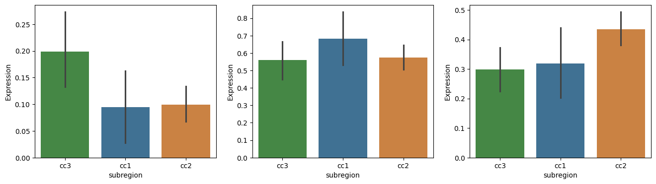
fig, axes = plt.subplots(nrows=1, ncols=3, figsize=(16, 4))
# top_genes_df_filt = top_genes_df[top_genes_df['logfoldchanges'] > 1]
cc = ['ctx1', 'ctx2', 'ctx3']
for i, cc_area in enumerate(cc):
    gene_data = adata_cc[:, top_genes_df.loc[cc_area]['gene']].X.A.mean(axis=1)
    group_data = adata_cc.obs['cc']
    df = pd.DataFrame({
        'Expression': gene_data,
        'subregion': group_data
    })
    ax = axes[i]
    sns.barplot(x='subregion', y='Expression', data=df, ax = ax, palette=['#3a923a', '#3274a1', '#e1812c'], order=['cc3', 'cc1', 'cc2'])

_images/9_ctx_3region_DEGs_expression_in_cc_14_0.png