3_ctx_th_connection_and_gene_correlation

[1]:

import pandas as pd
import scanpy as sc
from tqdm import tqdm
import matplotlib.pyplot as plt
import anndata as ad
import numpy as np
import warnings
from scipy.stats import pearsonr
import seaborn as sns
from scipy.cluster.hierarchy import fcluster, linkage
import matplotlib as mpl
mpl.rcParams['pdf.fonttype'] = 42
mpl.rcParams['ps.fonttype'] = 42

warnings.filterwarnings('ignore')

[2]:

adj = np.load('/mnt/Data18Td/Data/haichao/mouse_connect_data/NT/zxw/mouse_3/zxw_not_symmetric_adj.npy', mmap_mode='r')
print(adj.shape)

adata = sc.read_h5ad('/mnt/Data16Tc/home/haichao/code/SpaCon/ST_NT_cluster/SpaCon_apply_zxw/data/mouse_3/adata_merge.h5ad')
sc.pp.normalize_total(adata, target_sum=1e4)
sc.pp.log1p(adata)
allen_region = pd.read_csv('/mnt/Data16Tc/home/haichao/code/SpaCon/ST_NT_cluster/SpaCon_apply_zxw/data/mouse_3/allen_region.csv')
adata.obs['region'] = allen_region['region'].to_list()
adata.obs['spot_num'] = [i for i in range(adata.n_obs)]
adata

(107909, 107909)

[2]:

AnnData object with n_obs × n_vars = 107909 × 1122
    obs: 'x', 'y', 'z', 'section', 'NT_index', 'Cells_id', 'region', 'spot_num'
    uns: 'log1p'

subregion th ctx correlation

[3]:

th_regions = ['AD', 'AMd', 'AMv', 'AV', 'CL', 'CM', 'IAD', 'IAM', 'IGL', 'IMD', 'LD', 'LGv', 'LH', 'LP', 'MD', 'MGd', 'MGm', 'MGv', 'MH', 'PCN', 'PF', 'PIL', 'PO', 'POL',
                'PP', 'PR', 'PT', 'PVT', 'PoT', 'RE', 'RH', 'RT', 'SGN', 'SMT', 'SPA', 'SPFm', 'SPFp', 'VAL', 'VM', 'VPL', 'VPLpc', 'VPM', 'VPMpc', 'Xi']
ctx_regions = ['ACAd', 'ACAv', 'AId', 'AIp', 'AIv', 'AUDd', 'AUDp', 'AUDpo',
                'AUDv', 'ECT', 'FRP', 'GU', 'ILA', 'MOp', 'MOs', 'ORBl', 'ORBm',
                'ORBvl', 'PERI', 'PL', 'RSPagl', 'RSPd', 'RSPv', 'SSp-bfd',
                'SSp-ll', 'SSp-m', 'SSp-n', 'SSp-tr', 'SSp-ul', 'SSp-un', 'SSs',
                'TEa', 'VISC', 'VISa', 'VISal', 'VISam', 'VISl', 'VISli', 'VISp',
                'VISpl', 'VISpm', 'VISpor', 'VISrl']

adata_ctx_th_area = adata[(adata.obs['region'].str.startswith(tuple(ctx_regions))) | (adata.obs['region'].isin(th_regions))]
adata_ctx_th_area.obs['CT_spot_num'] = [i for i in range(adata_ctx_th_area.n_obs)]
adata_ctx_th_area.obs['ctx_or_th'] = 'nan'
for c in ctx_regions:
    adata_ctx_th_area.obs.loc[adata_ctx_th_area.obs['region'].str.startswith(c), 'ctx_or_th'] = 'ctx'
for c in th_regions:
    adata_ctx_th_area.obs.loc[adata_ctx_th_area.obs['region']==c, 'ctx_or_th'] = 'th'
adata_ctx_th_area.obs

[3]:

	x	y	z	section	NT_index	Cells_id	region	spot_num	CT_spot_num	ctx_or_th
2	19.113418	23.994053	46.894548	Zhuang-ABCA-3.005	2	188949490498702611647640449216501815503_304478...	FRP1	0	0	ctx
4	18.921382	24.017347	49.257099	Zhuang-ABCA-3.004	4	123445075025856302518661678660778224944_131347...	FRP1	1	1	ctx
6	19.079053	23.564575	51.258567	Zhuang-ABCA-3.003	6	319072152716142889780926524544977408256_106358...	FRP1	2	2	ctx
7	18.816739	25.041919	43.046671	Zhuang-ABCA-3.007	7	47102176527243727968506801819481818675_1792889...	FRP1	3	3	ctx
9	18.792692	25.077860	45.101231	Zhuang-ABCA-3.006	9	199428730039264634225478952930502449426_202483...	FRP1	4	4	ctx
...	...	...	...	...	...	...	...	...	...	...
148907	94.906133	15.937666	42.404653	Zhuang-ABCA-3.007	148907	106526352840576802488939912804342681931_107003...	RSPd1	75568	33095	ctx
148919	95.201531	17.993761	40.377543	Zhuang-ABCA-3.008	148919	133921573428284040813862276100319739380_145548...	RSPd1	75574	33096	ctx
148971	96.095220	15.844123	42.457680	Zhuang-ABCA-3.007	148971	149021058656557956290496348449572943108_174675...	RSPd1	75604	33097	ctx
148993	97.188915	11.409533	46.662115	Zhuang-ABCA-3.005	148993	107188929587695452503950023602364017291_167314...	RSPd1	75616	33098	ctx
193053	104.490816	24.420635	25.679869	Zhuang-ABCA-3.015	193053	43354620289828560228522986006306173486	VISpl1	99924	33099	ctx

33100 rows × 10 columns

[4]:

# Generate ROIs

mergecell_num = 20
def cluster_region(df_region, num_points=mergecell_num):
    # Perform hierarchical cluster
    Z = linkage(df_region[['x', 'y', 'z']], method='ward')
    # Divided into clusters according to the results of the cluster, each cluster has about NUM_POINTS individual points
    cluster_labels = fcluster(Z, t=len(df_region) / num_points, criterion='maxclust')
    return cluster_labels

# Initialize a empty cluster label
adata_ctx_th_area.obs['subregion'] = 0

# Perform clusters separately for each area
for region in adata_ctx_th_area.obs['region'].unique():
    mask = adata_ctx_th_area.obs['region'] == region
    if adata_ctx_th_area[adata_ctx_th_area.obs['region'] == region].shape[0] < 15:
        adata_ctx_th_area.obs.loc[mask, 'subregion'] = adata_ctx_th_area.obs.loc[mask, 'region'].apply(lambda x: x + '_1')
        continue

    clu_list = cluster_region(adata_ctx_th_area.obs[mask])
    cl_list = [f'{region}_{i}' for i in clu_list]
    adata_ctx_th_area.obs.loc[mask, 'subregion'] = cl_list

adata_ctx_th_area.obs

[4]:

	x	y	z	section	NT_index	Cells_id	region	spot_num	CT_spot_num	ctx_or_th	subregion
2	19.113418	23.994053	46.894548	Zhuang-ABCA-3.005	2	188949490498702611647640449216501815503_304478...	FRP1	0	0	ctx	FRP1_2
4	18.921382	24.017347	49.257099	Zhuang-ABCA-3.004	4	123445075025856302518661678660778224944_131347...	FRP1	1	1	ctx	FRP1_1
6	19.079053	23.564575	51.258567	Zhuang-ABCA-3.003	6	319072152716142889780926524544977408256_106358...	FRP1	2	2	ctx	FRP1_1
7	18.816739	25.041919	43.046671	Zhuang-ABCA-3.007	7	47102176527243727968506801819481818675_1792889...	FRP1	3	3	ctx	FRP1_2
9	18.792692	25.077860	45.101231	Zhuang-ABCA-3.006	9	199428730039264634225478952930502449426_202483...	FRP1	4	4	ctx	FRP1_2
...	...	...	...	...	...	...	...	...	...	...	...
148907	94.906133	15.937666	42.404653	Zhuang-ABCA-3.007	148907	106526352840576802488939912804342681931_107003...	RSPd1	75568	33095	ctx	RSPd1_3
148919	95.201531	17.993761	40.377543	Zhuang-ABCA-3.008	148919	133921573428284040813862276100319739380_145548...	RSPd1	75574	33096	ctx	RSPd1_3
148971	96.095220	15.844123	42.457680	Zhuang-ABCA-3.007	148971	149021058656557956290496348449572943108_174675...	RSPd1	75604	33097	ctx	RSPd1_3
148993	97.188915	11.409533	46.662115	Zhuang-ABCA-3.005	148993	107188929587695452503950023602364017291_167314...	RSPd1	75616	33098	ctx	RSPd1_2
193053	104.490816	24.420635	25.679869	Zhuang-ABCA-3.015	193053	43354620289828560228522986006306173486	VISpl1	99924	33099	ctx	VISpl1_2

33100 rows × 11 columns

[6]:

regions = adata_ctx_th_area.obs['subregion'].values
gene_expression = adata_ctx_th_area.X.A

# Create a DataFrame to integrate regional information and gene expression matrix together
df = pd.DataFrame(gene_expression, columns=adata.var_names)
df['subregion'] = regions

# Calculate the average gene expression by regional grouping and calculate the average gene
region_mean_expression = df.groupby('subregion').mean()
# Convert the result to the matrix format of the regional*gene
region_gene_matrix = region_mean_expression.values
region_gene_matrix.shape

[6]:

(1719, 1122)

[7]:

corr_all = np.corrcoef(region_gene_matrix)
corr_all.shape

[7]:

(1719, 1719)

[8]:

adata_th = adata_ctx_th_area[adata_ctx_th_area.obs['ctx_or_th'] == 'th']
th_subregions = adata_th.obs['subregion'].unique()
th_subregions.shape

[8]:

(244,)

[9]:

adata_ctx = adata_ctx_th_area[adata_ctx_th_area.obs['ctx_or_th'] == 'ctx']
ctx_subregions = adata_ctx.obs['subregion'].unique()
ctx_subregions.shape

[9]:

(1475,)

[10]:

region_labels = region_mean_expression.index
ctx_indices = [i for i, label in enumerate(region_labels) if label in ctx_subregions]
th_indices = [i for i, label in enumerate(region_labels) if label in th_subregions]
corr = corr_all[np.ix_(ctx_indices, th_indices)]
corr.shape

[10]:

(1475, 244)

[11]:

ctx_regions_df = [region_labels[i] for i in ctx_indices]
th_regions_df = [region_labels[i] for i in th_indices]
corr_df = pd.DataFrame(corr, index=ctx_regions_df, columns=th_regions_df)
corr_df

[11]:

	AD_1	AMd_1	AMd_2	AMv_1	AV_1	AV_2	AV_3	AV_4	AV_5	CL_1	...	VPM_23	VPM_3	VPM_4	VPM_5	VPM_6	VPM_7	VPM_8	VPM_9	VPMpc_1	VPMpc_2
ACAd1_1	0.596044	0.629380	0.629344	0.640548	0.625990	0.616779	0.625027	0.579291	0.607824	0.661248	...	0.546631	0.580518	0.560330	0.552390	0.588024	0.567292	0.550110	0.595391	0.673908	0.651029
ACAd2/3_1	0.597459	0.627501	0.638063	0.645888	0.624184	0.613061	0.610360	0.584868	0.599027	0.632073	...	0.563330	0.591786	0.587295	0.583098	0.590525	0.565894	0.574953	0.613022	0.647487	0.650415
ACAd2/3_2	0.571027	0.595831	0.606491	0.613162	0.593237	0.584572	0.577454	0.553500	0.566546	0.593970	...	0.539473	0.565224	0.567445	0.557278	0.561655	0.535150	0.554062	0.588653	0.610546	0.617166
ACAd2/3_3	0.553607	0.575565	0.594226	0.598235	0.573342	0.568132	0.569627	0.543022	0.554639	0.581051	...	0.514714	0.539524	0.537075	0.534365	0.534878	0.514530	0.527182	0.561045	0.591705	0.611740
ACAd5_1	0.630058	0.641793	0.647781	0.654390	0.634837	0.628741	0.631047	0.606152	0.623477	0.657897	...	0.572636	0.597883	0.591053	0.575654	0.597200	0.584400	0.576911	0.614796	0.669636	0.661564
...	...	...	...	...	...	...	...	...	...	...	...	...	...	...	...	...	...	...	...	...	...
VISrl4_1	0.608806	0.629851	0.637136	0.650792	0.617430	0.627219	0.614035	0.611263	0.604888	0.627469	...	0.577205	0.623548	0.610158	0.606235	0.613583	0.559556	0.614110	0.639994	0.649961	0.646791
VISrl5_1	0.649082	0.647604	0.668424	0.675256	0.653244	0.647948	0.637781	0.631115	0.636032	0.648355	...	0.617031	0.645198	0.637634	0.624230	0.644994	0.610415	0.630391	0.650415	0.684320	0.669412
VISrl5_2	0.643372	0.636174	0.654321	0.670814	0.631363	0.641428	0.625480	0.634172	0.618452	0.648326	...	0.587593	0.635670	0.617376	0.604309	0.627833	0.580243	0.623062	0.645508	0.675442	0.656189
VISrl6a_1	0.587644	0.558709	0.591176	0.606841	0.577877	0.581434	0.567537	0.566168	0.559256	0.581017	...	0.536177	0.560639	0.547816	0.527045	0.555997	0.526904	0.540306	0.558628	0.609119	0.590757
VISrl6b_1	0.657098	0.647202	0.689478	0.700880	0.679191	0.673361	0.654070	0.618012	0.638369	0.687741	...	0.614595	0.632637	0.627957	0.580900	0.653153	0.615239	0.588846	0.612918	0.721750	0.671169

1475 rows × 244 columns

connection

ctx2th conn

[12]:

ctx_ave_list = []
for c in tqdm(ctx_regions_df):
    adata_ctx_area = adata_ctx_th_area[adata_ctx_th_area.obs['subregion'] == c]

    # break
    idx = adata_ctx_area.obs['spot_num'].tolist()
    temp = np.mean(adj[idx], axis=0)
    ctx_ave_list.append(temp)
    # break
ctx2th_ave = np.vstack(ctx_ave_list)
ctx2th_ave.shape

100%|██████████| 1475/1475 [09:42<00:00,  2.53it/s]

[12]:

(1475, 107909)

[13]:

th_ave_list = []
for th_region in tqdm(th_regions_df):
    adata_th_area = adata_ctx_th_area[adata_ctx_th_area.obs['subregion'] == th_region]
    # break
    idx = adata_th_area.obs['spot_num'].tolist()
    # break
    temp = np.mean(ctx2th_ave[:, idx], axis=1)
    th_ave_list.append(temp)

ctx2th_ave = np.column_stack(th_ave_list)
conn_df = pd.DataFrame(data=ctx2th_ave, index=ctx_regions_df, columns=th_regions_df, dtype=float)
ctx2th_ave.shape

100%|██████████| 244/244 [00:00<00:00, 359.77it/s]

[13]:

(1475, 244)

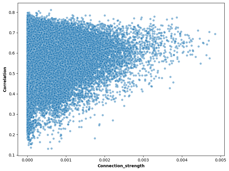
[14]:

corr = corr.flatten()
conn = ctx2th_ave.flatten()
plt.figure(figsize=(8, 6))
ax = sns.scatterplot(conn, corr, s=30, alpha=0.5)

plt.xlabel('Connection_strength', fontweight='bold')
plt.ylabel('Correlation', fontweight='bold')
plt.tight_layout()

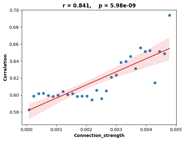
_images/3_ctx_th_connection_and_gene_correlation_16_0.png

[28]:

df = pd.DataFrame({'Correlation': corr,
                   'Connection_strength': conn})
# df = df[df['Connection_strength'] > 0.0005]
min_corr = df['Connection_strength'].min()
max_corr = df['Connection_strength'].max()
bins = np.linspace(0, max_corr, 31)
df['group'] = pd.cut(df['Connection_strength'], bins, include_lowest=False)

result = df.groupby('group')['Correlation'].median().reset_index()
result['Connection_strength'] = result['group'].apply(lambda x: (x.left + x.right) / 2)
result = result.dropna(subset=['Correlation'])

import scipy.stats as stats
correlation, p_value = pearsonr(result['Connection_strength'], result['Correlation'])
sns.regplot(data=result, x="Connection_strength", y="Correlation",
            scatter_kws={'s': 30, 'color': '#2878B5', 'alpha': 1, 'marker': 'o'},
            line_kws={'linewidth': 2, 'color': '#D8383A', 'linestyle': '-'})
slope, intercept, r_value, p_value, std_err = stats.linregress(result["Connection_strength"], result["Correlation"])
print(f"(slope): {slope}")
# plt.text(0.95, 0.01, f'Corr: {correlation:.2f}', ha='right', va='bottom', transform=plt.gca().transAxes)
plt.title(f'r = {correlation:.3f},    p = {p_value:.2e}', fontweight='bold')
plt.xlabel('Connection_strength', fontweight='bold')
plt.ylabel('Correlation', fontweight='bold')
plt.savefig('./th_ctx_corr_conn_scatter_line.pdf', format='pdf')
# plt.savefig(f'/mnt/Data16Tc/home/haichao/code/SpaCon/PaperFig/new_brief_comm_fig2/th_ctx_region_correlation/zxw3_all_40bins_merge{mergecell_num}cell.png', dpi=600)

斜率 (slope): 15.42913379110221

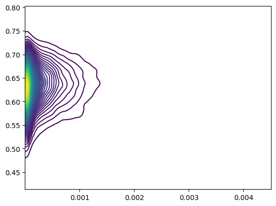
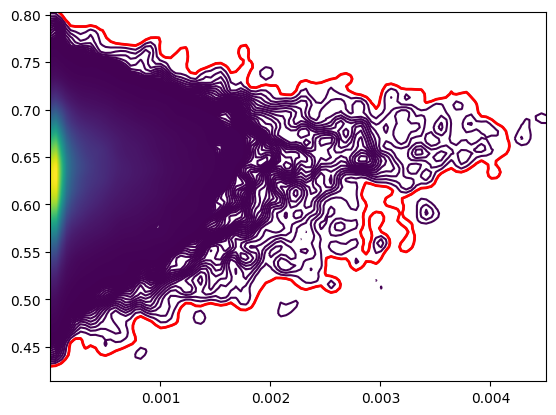
_images/3_ctx_th_connection_and_gene_correlation_17_1.png

[33]:

from scipy.stats import gaussian_kde

x = conn
y = corr

# Create a grid
xi, yi = np.mgrid[x.min():x.max():100j, y.min():y.max():100j]

# Calculate nuclear density estimation
positions = np.vstack([xi.ravel(), yi.ravel()])
values = np.vstack([x, y])
kernel = gaussian_kde(values)
z = np.reshape(kernel(positions).T, xi.shape)

# Draw scattered dots and outlines
fig, ax = plt.subplots()
# ax.scatter(x, y, c='k', alpha=0.3)
ax.contour(xi, yi, z, levels=100, cmap='viridis')

plt.show()

_images/3_ctx_th_connection_and_gene_correlation_18_0.png

[34]:

fig, ax = plt.subplots()

contour_set = ax.contour(xi, yi, z, levels=10000, cmap='viridis')

# Get the outermost contour (that is, the first outline)
outermost_contour = contour_set.collections[1]

# Extract the exterior outline path
paths = outermost_contour.get_paths()
outermost_path = paths[0]

# Draw the outermost outline
ax.plot(outermost_path.vertices[:, 0], outermost_path.vertices[:, 1], 'r-', linewidth=2)

plt.show()

# Get the coordinates of the outermost contour
outermost_contour_coords = outermost_path.vertices

Locator attempting to generate 8165 ticks ([0.0, ..., 32656.0]), which exceeds Locator.MAXTICKS (1000).

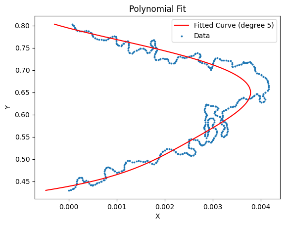
_images/3_ctx_th_connection_and_gene_correlation_19_1.png

[35]:

x_data = outermost_path.vertices[:, 1]
y_data = outermost_path.vertices[:, 0]

# Select the order of polynomial (you can adjust to get better fitting)
degree = 5

# Use Numpy's polynomial fitting
coeffs = np.polyfit(x_data, y_data, degree)
poly = np.poly1d(coeffs)

# Point to generate the fit curve
x_fit = np.linspace(min(x_data), max(x_data), 100)
y_fit = poly(x_fit)

# Draw the original data point and fit curve
plt.scatter(y_data, x_data, label='Data', s=3)
plt.plot(y_fit, x_fit, 'r-', label=f'Fitted Curve (degree {degree})')
plt.legend()
plt.xlabel('X')
plt.ylabel('Y')
plt.title('Polynomial Fit')
plt.show()

# Print polynomial coefficient
print("Polynomial coefficient (from high -level to low -level):")
for i, coeff in enumerate(coeffs):
    print(f"x^{degree-i}: {coeff:.4f}")

_images/3_ctx_th_connection_and_gene_correlation_20_0.png

多项式系数（从高阶到低阶）:
x^5: 12.8520
x^4: -39.7188
x^3: 48.3887
x^2: -29.1442
x^1: 8.7148
x^0: -1.0373

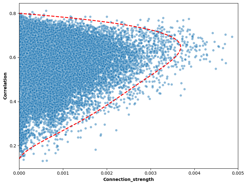
[97]:

plt.figure(figsize=(8, 6))
ax = sns.scatterplot(conn, corr, s=30, alpha=0.5)
ax.plot(y_fit, x_fit, 'r--', label=f'Fitted Curve (degree {degree})', linewidth=2)
plt.xlabel('Connection_strength', fontweight='bold')
plt.ylabel('Correlation', fontweight='bold')
plt.xlim(0, 0.005)
ax.set_xticks([0.000, 0.001, 0.002, 0.003, 0.004, 0.005])  # Set the X -axis scale
ax.set_yticks([0.2, 0.4, 0.6, 0.8])  # Set y -axial scale
plt.tight_layout()
# plt.savefig('./corr_conn_scatter.png', dpi=600)

_images/3_ctx_th_connection_and_gene_correlation_21_0.png

[ ]:

from scipy.stats import skew, kurtosis, normaltest, jarque_bera
# Polynomial coefficient (from high -level to low -level)
coefficients = coeffs

# Define the polynomial function
poly_func = np.poly1d(coefficients)

# Generate X value
x = np.linspace(min(x_data), max(x_data), 1000)
# Calculate the Y value of polynomial
data = poly_func(x)

# Calculation bias and peak degree
skewness = skew(data)
kurt = kurtosis(data) + 3  # Scipy's Kurtosis function returns the peak degree (Excess Kurtosis), you need to add 3 to get the peak degree

print(f"skewness: {skewness}")
print(f"kurt: {kurt}")

# D'Agostino's K-squared test
k2_stat, k2_p_value = normaltest(data)
print(f"D'Agostino's K-squared: {k2_stat}")
print(f"p: {k2_p_value}")


# Jarque-Bera test
jb_stat, jb_p_value = jarque_bera(data)
print(f"Jarque-Bera: {jb_stat}")
print(f"p: {jb_p_value}")

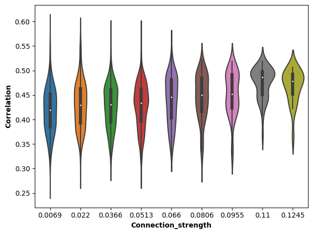
[17]:

df = pd.DataFrame({'Correlation': corr,
                   'Connection_strength': conn})

min_corr = df['Connection_strength'].min()
max_corr = df['Connection_strength'].max()
bins = np.linspace(min_corr, max_corr, 10)
df['group'] = pd.cut(df['Connection_strength'], bins, include_lowest=True)
df['Connection_strength'] = df['group'].apply(lambda x: round(((x.left + x.right) / 2), 4))
sns.violinplot(x='Connection_strength', y='Correlation', data=df)
plt.xlabel('Connection_strength', fontweight='bold')
plt.ylabel('Correlation', fontweight='bold')
plt.tight_layout()

_images/3_ctx_th_connection_and_gene_correlation_23_0.png