4_ctx_layer56_and_th_correlation

[1]:

import pandas as pd
import anndata
import scanpy as sc
from tqdm import tqdm
import matplotlib.pyplot as plt
import numpy as np
import warnings
import seaborn as sns
from scipy.cluster.hierarchy import fcluster, linkage
import matplotlib as mpl
mpl.rcParams['pdf.fonttype'] = 42
mpl.rcParams['ps.fonttype'] = 42
warnings.filterwarnings('ignore')

[2]:

ctx_regions = ['ACAd', 'ACAv', 'PL', 'ILA', 'ORBl', 'ORBvl', 'AId', 'SSs', 'SSp-bfd', 'SSp-ll', 'SSp-ul', 'SSp-n', 'SSp-m', 'MOp',
               'MOs', 'VISal', 'VISl', 'VISp', 'VISpor', 'VISrl', 'VISam', 'VISpm', 'RSPd', 'RSPv', 'AUDp']
th_regions = ['VPL', 'VPM', 'PO', 'PoT', 'VPMpc', 'VPLpc', 'SPFp',
              'MG', 'PIL', 'PP', 'SGN', 'AD', 'AV', 'LD', 'LP', 'VAL', 'PF', 'CL',
              'SubG', 'LGv', 'IGL', 'POL', 'MD', 'IMD', 'CM', 'SMT',
              'SPA', 'VM', 'PCN', 'PVT', 'PT', 'RE', 'SPFm', 'Xi', 'RH', 'IAM', 'PR',
              'LH', 'MH', 'IAD', 'RT']

[3]:

adata_raw = sc.read_h5ad('/mnt/Data16Tc/home/haichao/code/SpaCon/Data/N_20231213_zxw/mouse_3/adata_processed.h5ad')
allen_region = pd.read_csv('/mnt/Data16Tc/home/haichao/code/SpaCon/Data/N_20231213_zxw/mouse_3/allen_region.csv')
adata_raw.obs['region'] = allen_region['region'].values
# add cell type
meta = pd.read_csv('/mnt/Data16Tc/home/haichao/code/SpaCon/Data/N_20231213_zxw/mouse_3/cell_metadata_with_cluster_annotation.csv')
meta = meta.set_index('cell_label')
meta = meta.loc[adata_raw.obs.index.to_list()]
adata_raw.obs['cell_type'] = meta['class'].to_list()
adata_raw.obs

[3]:

	brain_section_label	x	y	z	x_ccf	y_ccf	z_ccf	region	cell_type
cell_label
198904341065180396762707397604803217407	Zhuang-ABCA-3.023	49.206853	44.877634	12.168155	4.920685	4.487763	1.216815	SSs1	33 Vascular
252199681526991424029643077826220097990	Zhuang-ABCA-3.023	48.973992	44.813761	12.179006	4.897399	4.481376	1.217901	SSs1	33 Vascular
277720971126854564514249564750701518375	Zhuang-ABCA-3.023	48.791066	44.577722	12.192707	4.879107	4.457772	1.219271	SSs1	33 Vascular
31551867344111790264292067056219852271	Zhuang-ABCA-3.023	48.830489	44.426120	12.195078	4.883049	4.442612	1.219508	SSs1	33 Vascular
131102494428104399865219008178262036485	Zhuang-ABCA-3.023	48.308843	43.028156	12.267879	4.830884	4.302816	1.226788	SSs1	34 Immune
...	...	...	...	...	...	...	...	...	...
318102106429791409781741726367984532777	Zhuang-ABCA-3.009	131.090716	69.334275	41.436743	13.109072	6.933427	4.143674	MDRNd	30 Astro-Epen
35262847161560382172299767067854387528	Zhuang-ABCA-3.009	131.216032	69.494070	41.351034	13.121603	6.949407	4.135103	MDRNd	33 Vascular
75415866509570969932943497000463821106	Zhuang-ABCA-3.009	131.415152	70.764504	40.800403	13.141515	7.076450	4.080040	sctd	24 MY Glut
12350978322417280063239916106423065862	Zhuang-ABCA-3.009	131.646167	71.182557	40.595995	13.164617	7.118256	4.059599	sctd	24 MY Glut
327554758863546024460748891922509519354	Zhuang-ABCA-3.009	131.658892	71.414675	40.501356	13.165889	7.141468	4.050136	sctd	24 MY Glut

1566842 rows × 9 columns

[4]:

adata_th = adata_raw[adata_raw.obs['region'].isin(th_regions)]
adata_th = adata_th[adata_th.obs['cell_type'].str.contains('Glut')]

adata_ctx = adata_raw[(adata_raw.obs['region'].str.startswith(tuple(ctx_regions))) & (adata_raw.obs['region'].str.contains('5|6'))]
adata_ctx = adata_ctx[adata_ctx.obs['cell_type'].str.contains('Glut')]
adata_ctx.obs

[4]:

	brain_section_label	x	y	z	x_ccf	y_ccf	z_ccf	region	cell_type
cell_label
29162871883387929795006067736640436040	Zhuang-ABCA-3.023	61.666898	42.255912	12.232613	6.166690	4.225591	1.223261	SSs5	01 IT-ET Glut
293032136699589827732370249746624703959	Zhuang-ABCA-3.023	62.396840	41.838307	12.216430	6.239684	4.183831	1.221643	SSs5	01 IT-ET Glut
169008133492981499504077797165914124518	Zhuang-ABCA-3.023	64.994841	40.394608	12.161029	6.499484	4.039461	1.216103	SSs5	01 IT-ET Glut
227494694293280194589855295428860091482	Zhuang-ABCA-3.023	64.498586	40.611089	12.175537	6.449859	4.061109	1.217554	SSs5	01 IT-ET Glut
33873656525375865261837620890496116573	Zhuang-ABCA-3.023	64.282103	41.059249	12.175800	6.428210	4.105925	1.217580	SSs5	01 IT-ET Glut
...	...	...	...	...	...	...	...	...	...
229580843941555951333299912014571135110	Zhuang-ABCA-3.009	97.429638	10.575478	38.381706	9.742964	1.057548	3.838171	VISp5	01 IT-ET Glut
248292745152448671917314233790662445907	Zhuang-ABCA-3.009	97.150793	11.549455	38.284627	9.715079	1.154945	3.828463	VISp5	01 IT-ET Glut
329636896424947842904418891891676096227	Zhuang-ABCA-3.009	97.098822	10.816952	38.350628	9.709882	1.081695	3.835063	VISp5	01 IT-ET Glut
210578552686403511812793479380810073674	Zhuang-ABCA-3.009	98.298868	11.674211	38.311367	9.829887	1.167421	3.831137	VISp5	01 IT-ET Glut
5967642066674772504918301827478668961	Zhuang-ABCA-3.009	98.354235	12.399570	38.259130	9.835423	1.239957	3.825913	VISp5	01 IT-ET Glut

60861 rows × 9 columns

[8]:

adata = anndata.concat([adata_ctx, adata_th])
adata.obs

[8]:

	brain_section_label	x	y	z	x_ccf	y_ccf	z_ccf	region	cell_type
cell_label
29162871883387929795006067736640436040	Zhuang-ABCA-3.023	61.666898	42.255912	12.232613	6.166690	4.225591	1.223261	SSs5	01 IT-ET Glut
293032136699589827732370249746624703959	Zhuang-ABCA-3.023	62.396840	41.838307	12.216430	6.239684	4.183831	1.221643	SSs5	01 IT-ET Glut
169008133492981499504077797165914124518	Zhuang-ABCA-3.023	64.994841	40.394608	12.161029	6.499484	4.039461	1.216103	SSs5	01 IT-ET Glut
227494694293280194589855295428860091482	Zhuang-ABCA-3.023	64.498586	40.611089	12.175537	6.449859	4.061109	1.217554	SSs5	01 IT-ET Glut
33873656525375865261837620890496116573	Zhuang-ABCA-3.023	64.282103	41.059249	12.175800	6.428210	4.105925	1.217580	SSs5	01 IT-ET Glut
...	...	...	...	...	...	...	...	...	...
137125155786416424728071422508382942054	Zhuang-ABCA-3.009	86.480430	34.094203	37.248728	8.648043	3.409420	3.724873	SGN	19 MB Glut
186321231466624970722021094909324401885	Zhuang-ABCA-3.009	86.443977	35.015822	37.291043	8.644398	3.501582	3.729104	POL	19 MB Glut
262284519603134366801326445274337827961	Zhuang-ABCA-3.009	86.388989	32.866518	37.212756	8.638899	3.286652	3.721276	SGN	19 MB Glut
33608739852097367198466784523454261485	Zhuang-ABCA-3.009	86.904204	34.752896	37.268567	8.690420	3.475290	3.726857	POL	19 MB Glut
303385550649730012456703013017610179856	Zhuang-ABCA-3.009	88.389510	37.024369	37.400811	8.838951	3.702437	3.740081	POL	19 MB Glut

71462 rows × 9 columns

[9]:

sc.pp.normalize_total(adata, target_sum=1e4)
sc.pp.log1p(adata)
adata

[9]:

AnnData object with n_obs × n_vars = 71462 × 1122
    obs: 'brain_section_label', 'x', 'y', 'z', 'x_ccf', 'y_ccf', 'z_ccf', 'region', 'cell_type'
    uns: 'log1p'

ctx layer56 th correlation

L5/L6 corr

[24]:

mergecell_num = 80
def cluster_region(df_region, num_points=mergecell_num):
    # Perform hierarchical cluster
    Z = linkage(df_region[['x', 'y', 'z']], method='ward')
    # Divided into clusters according to the results of the cluster, each cluster has about NUM_POINTS individual points
    cluster_labels = fcluster(Z, t=len(df_region) / num_points, criterion='maxclust')
    return cluster_labels

# Initialize a empty cluster label
adata.obs['subregion'] = 0
# Perform clusters separately for each area
for region in adata.obs['region'].unique():
    mask = adata.obs['region'] == region
    if adata[adata.obs['region'] == region].shape[0] < 80:
        adata.obs.loc[mask, 'subregion'] = adata.obs.loc[mask, 'region'].apply(lambda x: x + '_1')
        continue
    clu_list = cluster_region(adata.obs[mask])
    cl_list = [f'{region}_{i}' for i in clu_list]
    adata.obs.loc[mask, 'subregion'] = cl_list
adata.obs

[24]:

	brain_section_label	x	y	z	x_ccf	y_ccf	z_ccf	region	cell_type	subregion
cell_label
29162871883387929795006067736640436040	Zhuang-ABCA-3.023	61.666898	42.255912	12.232613	6.166690	4.225591	1.223261	SSs5	01 IT-ET Glut	SSs5_16
293032136699589827732370249746624703959	Zhuang-ABCA-3.023	62.396840	41.838307	12.216430	6.239684	4.183831	1.221643	SSs5	01 IT-ET Glut	SSs5_16
169008133492981499504077797165914124518	Zhuang-ABCA-3.023	64.994841	40.394608	12.161029	6.499484	4.039461	1.216103	SSs5	01 IT-ET Glut	SSs5_15
227494694293280194589855295428860091482	Zhuang-ABCA-3.023	64.498586	40.611089	12.175537	6.449859	4.061109	1.217554	SSs5	01 IT-ET Glut	SSs5_15
33873656525375865261837620890496116573	Zhuang-ABCA-3.023	64.282103	41.059249	12.175800	6.428210	4.105925	1.217580	SSs5	01 IT-ET Glut	SSs5_15
...	...	...	...	...	...	...	...	...	...	...
137125155786416424728071422508382942054	Zhuang-ABCA-3.009	86.480430	34.094203	37.248728	8.648043	3.409420	3.724873	SGN	19 MB Glut	SGN_1
186321231466624970722021094909324401885	Zhuang-ABCA-3.009	86.443977	35.015822	37.291043	8.644398	3.501582	3.729104	POL	19 MB Glut	POL_1
262284519603134366801326445274337827961	Zhuang-ABCA-3.009	86.388989	32.866518	37.212756	8.638899	3.286652	3.721276	SGN	19 MB Glut	SGN_1
33608739852097367198466784523454261485	Zhuang-ABCA-3.009	86.904204	34.752896	37.268567	8.690420	3.475290	3.726857	POL	19 MB Glut	POL_1
303385550649730012456703013017610179856	Zhuang-ABCA-3.009	88.389510	37.024369	37.400811	8.838951	3.702437	3.740081	POL	19 MB Glut	POL_1

71462 rows × 10 columns

[26]:

regions = adata.obs['subregion'].values
gene_expression = adata.X.A

# Create a DataFrame to integrate regional information and gene expression matrix together
df = pd.DataFrame(gene_expression, columns=adata.var_names)
df['subregion'] = regions

# Calculate the average gene expression by regional grouping and calculate the average gene
region_mean_expression = df.groupby('subregion').mean()
# Convert the result to the matrix format of the regional*gene
region_gene_matrix = region_mean_expression.values
region_gene_matrix.shape

[26]:

(867, 1122)

[27]:

corr_all = np.corrcoef(region_gene_matrix)
corr_all.shape

[27]:

(867, 867)

[28]:

adata_th = adata[adata.obs['region'].isin(th_regions)]
th_subregions = adata_th.obs['subregion'].unique()
th_subregions.shape

[28]:

(124,)

[29]:

adata_ctx = adata[adata.obs['region'].str.startswith(tuple(ctx_regions))]
ctx_subregions = adata_ctx.obs['subregion'].unique()
ctx_subregions.shape

[29]:

(743,)

[30]:

region_labels = region_mean_expression.index
ctx_indices = [i for i, label in enumerate(region_labels) if label in ctx_subregions]
th_indices = [i for i, label in enumerate(region_labels) if label in th_subregions]
corr = corr_all[np.ix_(ctx_indices, th_indices)]
corr.shape

[30]:

(743, 124)

[31]:

ctx_regions_df = [region_labels[i] for i in ctx_indices]
th_regions_df = [region_labels[i] for i in th_indices]
corr_df = pd.DataFrame(corr, index=ctx_regions_df, columns=th_regions_df)
corr_df

[31]:

	AD_1	AD_2	AD_3	AV_1	AV_2	AV_3	AV_4	CL_1	CL_2	CM_1	...	VPM_2	VPM_3	VPM_4	VPM_5	VPM_6	VPM_7	VPM_8	VPM_9	VPMpc_1	VPMpc_2
ACAd5_1	0.410782	0.399958	0.429878	0.389128	0.399872	0.379626	0.385972	0.433726	0.448486	0.418421	...	0.349622	0.392964	0.367910	0.383102	0.396261	0.393593	0.400477	0.395913	0.471805	0.461550
ACAd5_10	0.393125	0.382621	0.415251	0.376264	0.384030	0.365063	0.373579	0.424826	0.446542	0.411051	...	0.326493	0.371632	0.347403	0.361314	0.376664	0.377090	0.379626	0.376344	0.458214	0.458316
ACAd5_11	0.398234	0.380920	0.420792	0.413818	0.409845	0.394324	0.400633	0.455472	0.467039	0.445792	...	0.374350	0.416192	0.391017	0.403894	0.426616	0.423503	0.427803	0.423335	0.489865	0.486841
ACAd5_12	0.410527	0.393434	0.435584	0.420335	0.419085	0.401034	0.407594	0.460431	0.469367	0.445620	...	0.388494	0.428909	0.405853	0.419587	0.437670	0.435193	0.440099	0.432376	0.496598	0.487125
ACAd5_13	0.396818	0.378964	0.416866	0.407649	0.404479	0.390833	0.399343	0.460673	0.475524	0.454787	...	0.371024	0.411906	0.387836	0.398777	0.426981	0.425960	0.424657	0.425608	0.492338	0.495915
...	...	...	...	...	...	...	...	...	...	...	...	...	...	...	...	...	...	...	...	...	...
VISrl5_3	0.403946	0.392158	0.447694	0.412068	0.431390	0.391572	0.398629	0.458871	0.478694	0.423189	...	0.357283	0.430841	0.399325	0.415467	0.413560	0.410179	0.426174	0.418796	0.503235	0.475361
VISrl6a_1	0.353894	0.351150	0.377903	0.321932	0.336051	0.315114	0.315966	0.350315	0.362867	0.331669	...	0.279148	0.314711	0.289657	0.306511	0.303450	0.303453	0.311159	0.308828	0.377244	0.372180
VISrl6a_2	0.329470	0.328920	0.359324	0.318948	0.331033	0.303589	0.304252	0.347650	0.365771	0.318220	...	0.264400	0.316115	0.284581	0.302115	0.291393	0.287109	0.301932	0.298410	0.378667	0.372998
VISrl6a_3	0.350070	0.348513	0.380515	0.334510	0.347604	0.322965	0.320802	0.363974	0.382227	0.333347	...	0.267162	0.328005	0.294717	0.311189	0.304804	0.300980	0.316639	0.313798	0.396515	0.383178
VISrl6b_1	0.322910	0.323277	0.349623	0.307613	0.317701	0.302240	0.302237	0.339289	0.357366	0.312219	...	0.243223	0.289870	0.263871	0.276627	0.276174	0.275492	0.282320	0.282552	0.361067	0.364670

743 rows × 124 columns

[32]:

tempdf = pd.read_excel('./data/layer56_to_th_connection_strength.xlsx', index_col=0, sheet_name=None)
Rbp4_L5 = tempdf['Sheet1']
Ntsr1_Syt6_L6 = tempdf['Sheet2']

Rbp4_L5 = Rbp4_L5.replace('TN', -10)
Rbp4_L5.loc['SSs'] = Rbp4_L5.loc[['SSs-1', 'SSs-2']].mean(axis=0)
Rbp4_L5.loc['MOs'] = Rbp4_L5.loc[['MOs-1', 'MOs-2']].mean(axis=0)
Rbp4_L5 = Rbp4_L5.drop(['SSs-1', 'SSs-2', 'MOs-1', 'MOs-2'], axis=0)
# Rbp4_L5 = Rbp4_L5.loc[:, col_list]
Rbp4_L5 = Rbp4_L5.loc[ctx_regions]

Ntsr1_Syt6_L6 = Ntsr1_Syt6_L6.replace('TN', -10)
Ntsr1_Syt6_L6.loc['SSs'] = Ntsr1_Syt6_L6.loc[['SSs-1', 'SSs-2']].mean(axis=0)
Ntsr1_Syt6_L6.loc['MOs'] = Ntsr1_Syt6_L6.loc[['MOs-1', 'MOs-2']].mean(axis=0)
Ntsr1_Syt6_L6 = Ntsr1_Syt6_L6.drop(['SSs-1', 'SSs-2', 'MOs-1', 'MOs-2'], axis=0)
# Ntsr1_Syt6_L6 = Ntsr1_Syt6_L6.loc[:, col_list]
Ntsr1_Syt6_L6 = Ntsr1_Syt6_L6.loc[ctx_regions]

Ntsr1_Syt6_L6.shape

[32]:

(25, 44)

[33]:

connect_strength = pd.DataFrame(index=corr_df.index, columns=corr_df.columns, dtype=float)
connraw = (Rbp4_L5 + Ntsr1_Syt6_L6)/2
for ctx in tqdm(connraw.index):
    for th in connraw.columns:
        rows = connect_strength.index.str.startswith(ctx)
        cols = connect_strength.columns.str.startswith(th)
        connect_strength.loc[rows, cols] = connraw.loc[ctx, th]

100%|██████████| 25/25 [00:00<00:00, 52.47it/s]

[37]:

ctx_region_order = ['ACAd', 'ACAv', 'PL', 'ILA', 'ORBl', 'ORBvl', 'AId', 'SSs', 'SSp-bfd', 'SSp-ll', 'SSp-ul', 'SSp-n', 'SSp-m', 'MOp', 'MOs', 'VISal', 'VISl', 'VISp', 'VISpor', 'VISrl', 'VISam', 'VISpm', 'RSPd', 'RSPv', 'AUDp']

[ ]:

tp = []
tn = []
for c in ctx_region_order:
    tmp = pd.DataFrame()
    tmp['conn'] = connect_strength.loc[connect_strength.index.str.startswith(c)].values.flatten()
    tmp['corr'] = corr_df.loc[corr_df.index.str.startswith(c)].values.flatten()
    tmp_p = tmp[(tmp['conn'] > -2)]
    # top_indices = tmp['conn'].nlargest(10).index
    # tmp_p = tmp.loc[top_indices]
    tmp_n = tmp[tmp['conn'] == -10]
    tp.append(tmp_p['corr'].mean())
    tn.append(tmp_n['corr'].mean())
values = tp
values2 = tn
feature = ctx_region_order

N = len(values)
# Set the angle of the radar diagram to cut a round surface in a flat separation
angles=np.linspace(0, 2*np.pi, N, endpoint=False)
# In order to close the radar map, the following steps need
values=np.concatenate((values,[values[0]]))
values2=np.concatenate((values2,[values2[0]]))
angles=np.concatenate((angles,[angles[0]]))
feature = np.concatenate((feature, [feature[0]]))
fig=plt.figure(figsize=(6,6))
ax = fig.add_subplot(111, polar=True)
# Draw a line map
ax.plot(angles, values, 'o-', markersize=2, linewidth=0.5, label = 'TP', color='#E56F5E')
# Fill color
ax.fill(angles, values, alpha=0.25, color='#F19685')
# Draw the second folding drawing
ax.plot(angles, values2, 'o-', markersize=2, linewidth=0.5, label = 'TN', color='#8d8d8d')
ax.fill(angles, values2, alpha=0.25, color='#8d8d8d')
# Add the tags of each feature
# ax.set_thetagrids(angles * 180/np.pi, feature)
ax.set_thetagrids(angles * 180/np.pi, feature)  # FRAC parameter setting label distance MAX ( *TP, *TN)+0.05 to depart the center
ax.tick_params(axis='x', pad=6)  # Set the distance between the label and the axis
# Set the range of radar chart
# ax.set_ylim(min(*tp, *tn)-0.05, max(*tp, *tn)+0.05)
ax.set_ylim(0.25, 0.45)
# Add title
# plt.title(f'Layer5/6_CTX_in & TH_in', fontweight='bold')
# Add grid line
# ax.grid(True)
ax.grid(True, linewidth=0.25, alpha=0.7)

# ax.set_rgrids([0.25, 0.3, 0.35, 0.4, 0.45], labels=['', '0.3', '', '0.4', ''])
# Set diagram
plt.legend(loc='center left', bbox_to_anchor=(1, 1))

plt.tight_layout()
# plt.savefig('./l56_module_ave_exp_radar_plot_out.pdf', format='pdf')

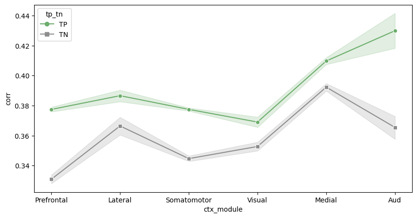
[109]:

ctx_module = {'Prefrontal': ['ACAd', 'ACAv', 'PL', 'ILA', 'ORBl', 'ORBvl'], 'Lateral': ['AId'], 'Somatomotor' :['SSs', 'SSp-bfd', 'SSp-ll', 'SSp-ul', 'SSp-n', 'SSp-m', 'MOp', 'MOs'],
              'Visual': ['VISal', 'VISl', 'VISp', 'VISpor', 'VISrl'], 'Medial': ['VISam', 'VISpm', 'RSPd', 'RSPv'], 'Aud': ['AUDp']}
# Reset the index to ensure that the index is listed as a column
df1_reset = connect_strength.reset_index()
df2_reset = corr_df.reset_index()
# Merge Dataframe
merged_df = df1_reset.melt(id_vars=['index'], var_name='th_region', value_name='conn')
merged_df['corr'] = df2_reset.melt(id_vars=['index'], var_name='th_region', value_name='corr')['corr']
# Huge naming
merged_df.rename(columns={'index': 'ctx_region'}, inplace=True)

merged_df['ctx_module'] = 0
for i, c in enumerate(ctx_module.keys()):
    merged_df.loc[merged_df['ctx_region'].str.startswith(tuple(ctx_module[c])), 'ctx_module'] = c

merged_df['tp_tn'] = 0
merged_df.loc[merged_df['conn'] > -2, 'tp_tn'] = 'TP'
merged_df.loc[merged_df['conn'] == -10, 'tp_tn'] = 'TN'
merged_df = merged_df[merged_df['tp_tn'] != 0]

plt.figure(figsize=(10,5))
order = ['Prefrontal', 'Lateral', 'Somatomotor', 'Visual', 'Medial', 'Aud']
merged_df['ctx_module'] = pd.Categorical(merged_df['ctx_module'], categories=order, ordered=True)
custom_palette = {
    'TP': '#6bad6b',
    'TN': '#8d8d8d'
}
# Custom label style
custom_markers = {
    'TP': 'o',  # Circle label
    'TN': 's'   # Square label
}
sns.lineplot(data=merged_df, x="ctx_module", y="corr", hue="tp_tn", style="tp_tn", markers=custom_markers, dashes=False, palette=custom_palette)
# sns.lineplot(data=merged_df, x="ctx_module", y="corr", hue="tp_tn", err_style="bars")
# plt.savefig('./L56_Moudel_tp_tn_compare_line.pdf', format='pdf')

[109]:

<AxesSubplot:xlabel='ctx_module', ylabel='corr'>

_images/4_ctx_layer56_and_th_correlation_20_1.png